The tutorial for using the DICe GUI and stereo DIC has not yet been released. Below are some tutorials for 2D full-field DIC and object tracking using the command line interface for DICe.

Introduction

This tutorial walks the user through several simple examples using DICe to do the following

Track parts inside a mechanism filmed with high speed video
Track objects in an image sequence that become obstructed
Compute strains in an object undergoing deformation

In all cases, the input files for these examples are located in the dice_root/examples folder if a package installer was used ton install DICe, or in the dice_root/tests/examples folder if referencing the source code. To experiment with these examples, these files should be copied to a temporary folder. Run the dice executable in the temporary folder rather than inside the repository or the system install directory.

Input Files

input.xml
params.xml
subsets.txt

The documentation describes how to generate input files for a DICe analysis. There are three files needed (two of which are optional) in addition to the image files or video file. The first is the input xml file, typically named input.xml. This file defines the images to analyze and the file locations, the frames to use, and optionally defines a parameters file (typically named ‘params.xml’). The parameters xml file defines the methods to use during the analysis and the method options. If no parameters file is specified, a set of default parameters is used. The names for each of the files above can be different than the suggested name, as long as the correct file name is referenced. The subset file defines the geometry of conformal subsets. In many cases, the subset file is not needed and the step size and subset size can simply be given in the input file. In other cases, for example when the objects studied have an oblong or odd shape, subsets that map to the edges of the object need to be used.

In each of the examples below, the input files are provided in the example directory. These can be used as a starting point for developing the input files for a more complicated analysis. Gold copies of the results files are also included with each of the examples. These files contain the expected solution for the given example.

To run any of the examples below, simply use a terminal or command line program to cd into the example directory and run the dice executable. On Mac the call would be:

<path_to_dice_exec>/dice -i input.xml -v -t

On Windows the call is:

<path_to_dice_exec>\dice.exe -i input.xml -v -t

The -v option turns on verbose output and the -t option will print the timing statistics.

Example 1: Mechanism

This example illustrates how to define conformal subsets and use them to track parts of a mechanism during operation.

The image data for this example is a .cine video file. The .cine format is used for high speed video. There are a number of problems with the image data for this example: the speckle pattern is not evenly distributed; the speckles are of poor sizes; the parts in the video move in a jerky fashion; the center wheel has a lot of speckular reflection; some parts are too small for a proper subset; and some parts are of odd shapes, making square subsets difficult. This example is designed to show how to collect motion data, even with a terrible set of images. It is definitately not a good example to follow in terms of the experimental set up.

The files for this example are in the mechanism folder of the tests/examples/ directory. The subsets are defined in the file subsets.txt and are shown in the image below. In the first section of the file, the coordinates of the centroid for each subset are defined. In this case, there are 4 subsets (ids:0,1,2,3). Notice several things about the subset definitions. The first is that two disconnected shapes are used to define Subset 0. Any number of shapes can be combined into a single subset. The shapes do not have to be contiguous. Also notice that the circular subset for subset 2 is only 5 pixels in radius. The results for this subset are less accurate than the rest due to the small subset size, but the u and v displacements can still be tracked relatively accurately. After plotting the results from each subset, the varying levels of confidence in the solution can be determined by comparing SIGMA, GAMMA, and BETA values. See the main documentation for the descriptions of what each of these fields represents.

Conformal subset definitions are not required for every subset. As long as the user has defined a subset_size in the input.xml file, any subsets that do not have a conformal_subset definition will be assigned a square region of the default dimensions.

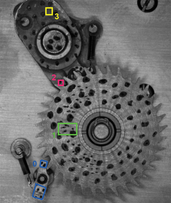
Another thing to notice is that Subset 3 is defined in a region that does not have any speckles! The reason that Subset 3 tracks without the need for speckles is because the SIMPLEX method is used as the correlation_method in params.xml. The SIMPLEX method does not rely on image gradients, hence speckles are not necessary. Speckles do however provide more accuracy, when the SIMPLEX method is used because it increases the contrast variation in the subset. Also without speckles the results are more prone to speckular reflection as the parts move. We include this speckle free subset here to show how DICe can be used to track motion without patterning.

Also included in the examples folder is a python script that will plot the results for each frame and subset. The script serves as a template to plot the results of individual subset motions or the full-field displacements.

Example 2: Obstructions

The files for this example are in the obstruction folder of the tests/examples/ directory.

This example shows how to manage obstructions that may block the path of the object being tracked. In some instances a subset will partially disappear behind an object. Most tracking algorithms will fail if this happens for even part of the subset. In DICe, these obstructions can be masked out (and even tracked themselves) so that the correlation only uses the visible portions of the subset.

For this example, a sequence of .tiff images is analyzed, rather than a .cine video. To analyze an image sequence with file names that have a structure similar to <image_file_prefix>_frame.<image_file_extension>, in input.xml the user can define the parts of the naming convention, as well as the reference frame number and the number of images to include. See the input file for an example of this.

Three things can be defined in the subset file that help with obstructions, two of which are optional. The first is the boundary definition (just like a normal subset). The second is an excluded are definition. These are parts of the subset that are either obstructed from view in the first frame or they can represent holes or breaks in the object being tracked. Pixels in excluded regions are deactivated for the first frame, i.e. they do not contribute to the correlation calculations. The pixels will stay deactivated throughout the analysis unless the user requests the use_subset_evolution option the params file. With this option, as the subset moves and pixels that were initially excluded come into view, they become activated. The intensity value for the reference pixel that was hidden during the first frame is determined by taking the average over several steps of the intensity value for the newly visible pixel in the deformed images.

The last region to be defined in the subset file is the obstructed region. These are fixed regions (that do not move in the video) that block portions or potentially block portions of a subset. Interactions between subsets that cross each other's paths are specified in the BLOCKING_SUBSETS command in the subset file.

The subsest defined in this example are shown in the figure below:

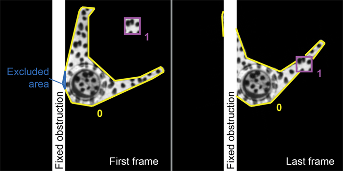
As Subset 0 rotates behind the fixed obstruction, the pixels that become blocked are deactivated. If the user changes the parameter for output_deformed_subset_images to true, images will be written for each step that show the deactivated pixels as white in color. The same is true for the parts of Subset 0 that become blocked by Subset 1 in the later frames.

The excluded area, shown in blue above, is also deactivated from the first frame because it is blocked by the fixed obstruction.

In the results for this example, a separate output file was generated for each subset. To split the subset solutions into their own files the separate_output_file_for_each_subset was used in input.xml.

Example 3: Full-field displacements and strains

The files for this example are in the full_field folder of the tests/examples/ directory.

This example shows how to perform a standard full-field DIC analysis and compute strains based on the displacements using the virtual strain gauge (VSG).

For this example, only two images are analyzed, a reference and deformed image. This is reflected in the input.xml file which has a slightly different structure than the input files above. In this case we do not have a sequence of images with a similar structure or a video file, but rather a list of images. More images can be added to the deformed_images list by specifying the file name. To disable processing any of the images in the list, simply change the boolean value to false rather than true.

The initialization_method for this example has been set to USE_NEIGHBOR_VALUES. When this method is used, each subset will be analyzed in an order that branches out from one subset, using the solution from a prior subset to initialize the next. An optional seed can be secified for the initial guess for the first subset if the deformations are large.

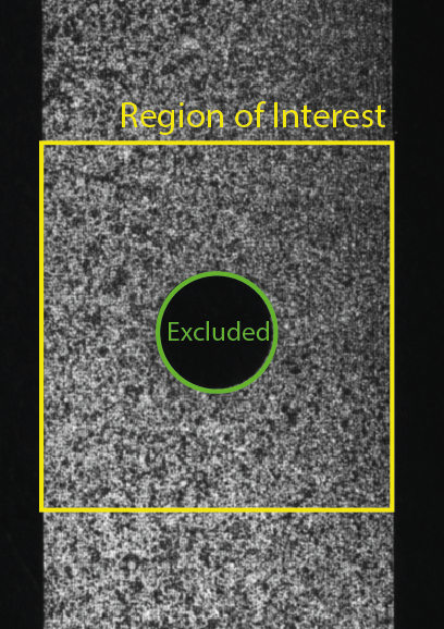
Rather than define specific subsets, in this example, a region_of_interest is defined in subsets.txt. This region has a rectangular section with a circle excluded from the center to omit the hole in the sample. See the image below.

The VSG strains are computed by adding the post_process_vsg_strain option to params.xml. The size of the virtual strain gauge window can be set by changing the sub-parameters in this section of params.xml.

In the results for this example, a single file holds the solution for all the subsets in the analysis (unlike the tracking examples above, where a separate file is produced for each subset).